Play Ball!
I think some of the appeal that baseball has always had for me comes from the data and stats that are intertwined in the game. I grew up playing little league and supporting the Seattle Mariners (sorry Jays, west coast proximity factor). I went to my first MLB game in 2001 at Safeco Field and instantly fell in love with the magic of the big leagues. More than just the hot dogs and garlic fries at the ballpark, I found my attention constantly being drawn to the player’s stats - batting averages, doubles, triples, home runs - displayed prominently on the Jumbotron scoreboard, and the giant LED pitch speed clocks scattered around the park. In 2011, I watched Moneyball with my dad, and like many others, was fascinated by the analytical approach that teams were beginning to take to gain a competitive edge in professional baseball. Although my support for the Mariners has not changed since that first day at the ballpark, the way I began to view stats did. I stumbled upon the world of sabermetrics and began to talk about players in terms of on-base percentage (OBP) and wins above replacement (WAR), instead of the traditional counting stats like hits and RBIs.

Now that I am beginning to learn R, my interest for exploring these stats and creating informative visualizations has been amplified. I figured it would be useful exercise to derive some of the modern baseball statistics like Weighted Runs Created Plus (wRC+) and FIP (Fielding Independant Pitching) from counting stats like hits and walks. There are great packages like baseballr that scrape this information for use but I wanted to have a go at it from first principles for the benefit of my understanding, so that’s what I’ll present here. The lahman package in R does not yet contain data from the 2017 so instead I’ll manually grab the csv files I need from the appropriate github repo. Necessary constants and weights will be obtained from FanGraphs. I haven’t had any experience scraping HTML tables yet so this will be done using the less glamorous export to csv functions on the website. Once I have all of the necessary tables, I use dplyr and its excellent relational table functions to extract and combine all of the information I need. Then comes the big mutate code block where I calculate all of the statistics. For an explanation of some of the more complicated ones, see below. Here is a sample of the lahman ‘Batting’ database.
Lahman Batting Database
## # A tibble: 20 x 22
##    playerID yearID stint teamID lgID      G    AB     R     H  `2B`  `3B`
##    <chr>     <dbl> <dbl> <chr>  <chr> <dbl> <dbl> <dbl> <dbl> <dbl> <dbl>
##  1 blackch~   2017     1 COL    NL      159   644   137   213    35    14
##  2 altuvjo~   2017     1 HOU    AL      153   590   112   204    39     4
##  3 gordode~   2017     1 MIA    NL      158   653   114   201    20     9
##  4 inciaen~   2017     1 ATL    NL      157   662    93   201    27     5
##  5 hosmeer~   2017     1 KCA    AL      162   603    98   192    31     1
##  6 andruel~   2017     1 TEX    AL      158   643   100   191    44     4
##  7 ozunama~   2017     1 MIA    NL      159   613    93   191    30     2
##  8 abreujo~   2017     1 CHA    AL      156   621    95   189    43     6
##  9 lemahdj~   2017     1 COL    NL      155   609    95   189    28     4
## 10 arenano~   2017     1 COL    NL      159   606   100   187    43     7
## 11 ramirjo~   2017     1 CLE    AL      152   585   107   186    56     6
## 12 schoojo~   2017     1 BAL    AL      160   622    92   182    35     0
## 13 vottojo~   2017     1 CIN    NL      162   559   106   179    34     1
## 14 lindofr~   2017     1 CLE    AL      159   651    99   178    44     4
## 15 cainlo01   2017     1 KCA    AL      155   584    86   175    27     5
## 16 murphda~   2017     1 WAS    NL      144   534    94   172    43     3
## 17 garciav~   2017     1 CHA    AL      136   518    75   171    27     5
## 18 jonesad~   2017     1 BAL    AL      147   597    82   170    28     1
## 19 yelicch~   2017     1 MIA    NL      156   602   100   170    36     2
## 20 merriwh~   2017     1 KCA    AL      145   587    80   169    32     6
## # ... with 11 more variables: HR <dbl>, RBI <dbl>, SB <dbl>, CS <dbl>,
## #   BB <dbl>, SO <dbl>, IBB <dbl>, HBP <dbl>, SH <dbl>, SF <dbl>,
## #   GIDP <dbl>
batting_processed <- batting %>%
left_join(teams %>% select(teamID, yearID, name, BPF), by = c("teamID", "yearID")) %>%
left_join(wrc_chart, by = c("yearID", "lgID")) %>%
left_join(woba_weights, by = c("yearID" = "Season")) %>%
mutate(PA = AB + BB + IBB + SH + SF + HBP,
TB = H + `2B` + 2 * `3B` + 3 * HR,
BA = ifelse(AB > 0, round(H/AB, 3), NA),
OBP = ifelse(AB > 0, round((H + BB + IBB + HBP)/PA, 3), NA), #ifelse statement deals with AB = 0 case
SA = ifelse(AB > 0, round(TB/AB, 3), NA),
OPS = OBP + SA,
slash = ifelse(!is.na(BA), paste(BA, OBP, SA, sep = "/"), NA),
BABIP = ifelse(AB > 0, round((H-HR)/(AB-SO-HR+SF), 3), NA),
wOBA = ifelse(AB > 0, (wBB*(BB-IBB) + wHBP*HBP + w1B*(H-`2B`-`3B`-HR) + w2B*`2B` + w3B*`3B` + wHR*HR) /(AB + BB - IBB + SF + HBP), NA),
wRAA = round(((wOBA - wOBALeague)/wOBAScale) * PA, 0),
WRC = round((wOBA - wOBALeague)/wOBAScale + RPALeague*PA, 0),
BPF = BPF/100, #BPF needs to be a fraction of 1 for calculations.
WRCplus = round((((wRAA/PA + RPALeague) + (RPALeague - BPF*RPALeague))/(wRCLeague/PALeague)*100), 0),
wOBA = round(wOBA, 3)) %>%
select(-(name:RPALeague)) #drop weight variables when we're finished
batting_processed <- batting_processed %>% #add in readable names from players database
left_join(players %>% select(playerID, nameFirst, nameLast), by = "playerID") %>%
mutate(Name = paste(nameLast, nameFirst, sep = ", ")) %>%
select(-nameFirst, -nameLast)Let me unpack the code chunk above a little bit. The batting database comes with a number of counting statistics from which all other statistics can be calculated. These are:
- AB: At Bats
- H: Total Hits
- 2B
- 3B
- HR
- BB: Walks (Base on Balls)
- IBB: Intentional Walks
- HBP: Hit by Pitch
- SH: Sacrifice Hits
- SF: Sacrifice Flies
From these we are able to calculate statistics that give us a better idea of a player’s value to their team. For a full explanation, each term links to the FanGraphs glossary page which includes the equation for its calculation as well as examples.
BABIP: Batting Average on Balls in Play - When we compare this value to a player’s batting average overall, we get a sense of how lucky or unlucky a player has been. I.e. when playing against a team with better defensive players this will be lower because they would make outs on plays that may normally drop in for a hit.
wOBA: Weighted on-base average gives empirical weights to each possible outcome a batter can have instead of assigning 1 to a single, 2 to a double, etc.
wRAA: Weighted Runs Above Average is a stat that attempts to quanitfy how many more runs a player contributed to their team than an average player would. This value can be negative or positive and uses the same weighting values as wOBA. The underlying principle behind sabermetrics is that if we can effectively quantify how many extra runs a player is worth, then we can infer how many extra wins a player can contribute to a team, the ultimate goal.
wRC+: Takes wRAA values and adjusts them for the current years’ run scoring environment as well as the hitter friendliness of the home park that they play in. It is also adjusted so that a WRC+ of 100 is league average, and someone with a wRC+ of 130 is considered to have had a 30% greater season at the plate than average.
One problem that I am still working on dealing with in this process is players that spent time with multiple teams during one season. These stints are each given a separate entry in the batting database and will need to be aggregated while accounting for different ball park factors etc. when calculating things like WRC+. With these stats we can start to imagine visualizations that we can create that contain much more information than something like home run or stolen base leaderboards.
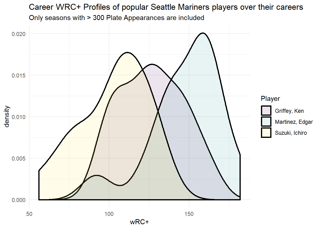
I’ll present a couple of examples to give an idea of some of the directions we can explore with this dataset. The first one is the WRCplus profile of a trio of Seattle Mariner greats across their careers. Edgar and Griffey were perennial power and gap hitters, whereas Ichiro was more of a singles hitter and speedster. As we can see, the WRC+ metric seems to favour the power hitter profile, something worth exploring in later posts.
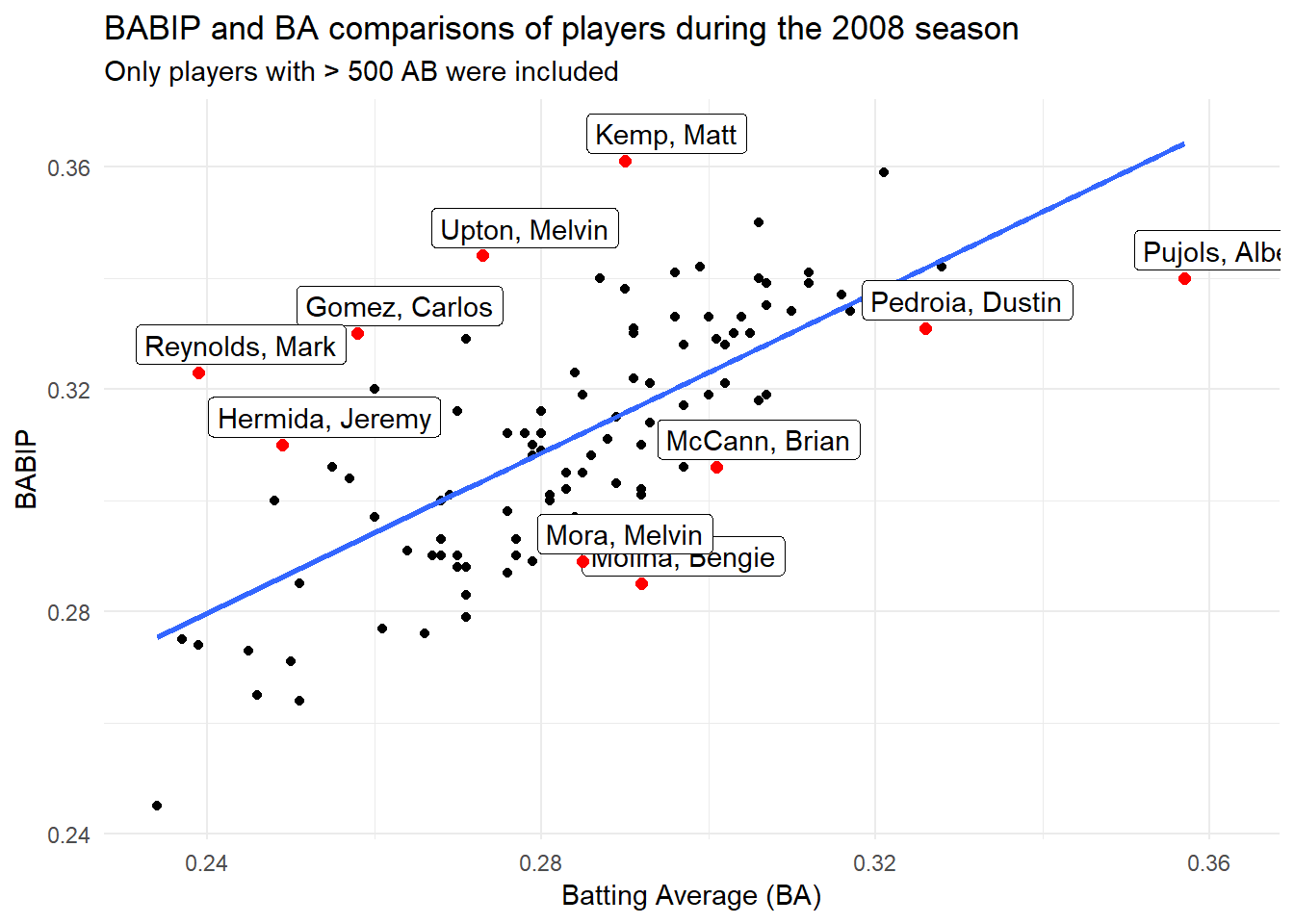
This next graph highlights the BABIP metric for the 2008 season, which if you recall can be thought of as a proxy for how lucky/unlucky a player has been in a season. I’ve added labels to the top 5 luckiest & unluckiest players based on a ratio of BABIP/BA. Players above the regression line were generally luckier than those below.
This ended up being mostly about Batting stats, so I will make a separate post addressing some of the popular modern pitching statistics and how to calculate them using publically available data. Future posts will dive a bit deeper into some player analysis, and predictive modelling for the upcoming 2019 season. As always, code & data will be available on my Github if you would like to explore for yourself.