Shiny is a fantastic tool for a number of reasons. For one, it is a platform to bring your data visualizations and results to life, and because it is hosted at shinyapps.io, sharing is as easy as copy and pasting a url to invite colleagues/friends/family to view your work. Most importantly however, is that it allows the end user to interact with your data, asking their own questions and coming to their own conclusions. This level of involvedness is crucial for retaining people’s attention, something that is becoming more and more difficult in modern society. Many examples of shiny apps that I have come across are incredibly versatile too, even allowing the user to upload their own dataset for analysis.

My shiny journey began at DataCamp, where I took the course “Building Web Applications in R with Shiny” as well as the case studies follow-up. These courses did an excellent job explaining concepts such as reactivity that are difficult for someone who does not have prior web development experience (me). After these courses I felt confident enough to jump into my own web application, which can be found here if you want to jump ahead!

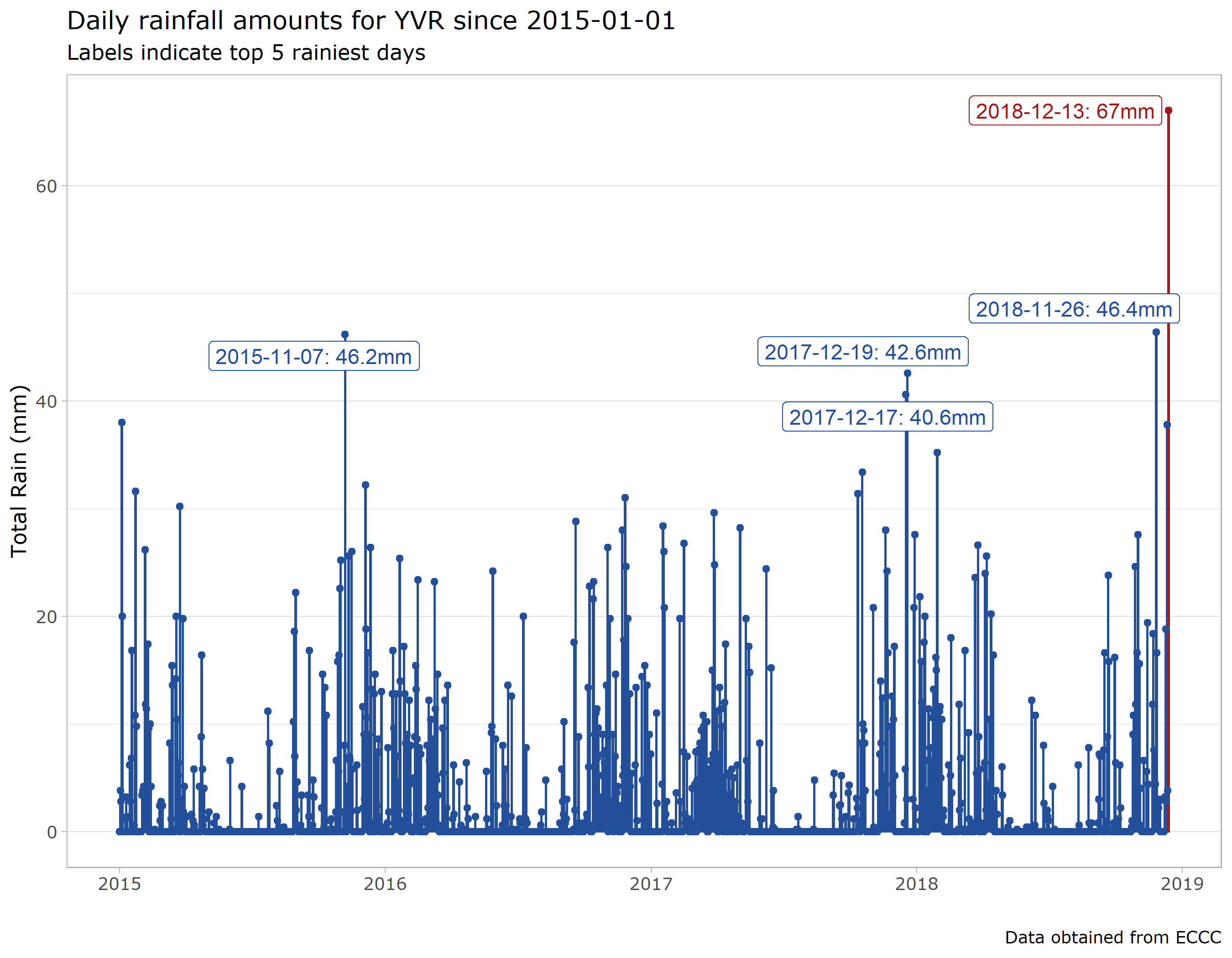
First, I needed an idea. My brother is a meteorologist with The Weather Network, and operator of the prolific PNW weather twitter account @50ShadesofVan. Recently, we have been collaborating to produce some informative graphics for his twitter audience such as those shown below (We’ve had an exceptional amount of rain on the west coast this winter):

So my premise was to create a simple app that allowed a user to compare historic temperature and precipitation trends across major Canadian cities using Environment Canada data. I relied heavily on the weathercan package to fetch my climate data from ECCC. Using the main function weather_dl a typical query for data was as follows:

library(weathercan)

weather_dl(station_ids = "51442", start = "2018-12-01", end = "2018-12-02", interval = "hour") %>%
  head(5)

## # A tibble: 5 x 35
##   station_name station_id station_operator prov    lat   lon  elev
##   <chr>        <chr>      <chr>            <fct> <dbl> <dbl> <dbl>
## 1 VANCOUVER I~ 51442      NAV Canada       BC     49.2 -123.   4.3
## 2 VANCOUVER I~ 51442      NAV Canada       BC     49.2 -123.   4.3
## 3 VANCOUVER I~ 51442      NAV Canada       BC     49.2 -123.   4.3
## 4 VANCOUVER I~ 51442      NAV Canada       BC     49.2 -123.   4.3
## 5 VANCOUVER I~ 51442      NAV Canada       BC     49.2 -123.   4.3
## # ... with 28 more variables: climate_id <chr>, WMO_id <chr>, TC_id <chr>,
## #   date <date>, time <dttm>, year <chr>, month <chr>, day <chr>,
## #   hour <chr>, weather <chr>, hmdx <dbl>, hmdx_flag <chr>,
## #   pressure <dbl>, pressure_flag <chr>, rel_hum <dbl>,
## #   rel_hum_flag <chr>, temp <dbl>, temp_dew <dbl>, temp_dew_flag <chr>,
## #   temp_flag <chr>, visib <dbl>, visib_flag <chr>, wind_chill <dbl>,
## #   wind_chill_flag <chr>, wind_dir <dbl>, wind_dir_flag <chr>,
## #   wind_spd <dbl>, wind_spd_flag <chr>

Data returned includes hour by hour information on pressure, humidity, temperature, and wind. If the interval variable is set to “day” in the weather_dl function, daily precipitation values are included. I chose to stick to temperature and precipitation for the purposes of my simple app. I used tidyverse tools to clean the data and extract variables that I knew I would want.

Trial and Error with Shiny

It’s amazing how much you can learn just by reading help documentation for functions and the subsequent error messages when you try and put them into practice. This process describes my initial experience with setting up user inputs and graph/table outputs with Shiny.

My first issue came up because I wanted to give the user the option to view daily data, or to average over monthly & yearly periods. In essence I wanted to perform different transformations on my dataset based on the input selected by the user. After some googling, I found an elegant solution using the switch function. In the UI function, I included a simple radio button input to let the user select the frequency of observations:

radioButtons(inputId = "freq", 
             label = "Frequency",
             choices = c("Daily" = "daily",
                         "Monthly" = "monthly",
                         "Yearly" = "yearly"),
             selected = "daily")

In the server function, I utilized the switch function to set up a reactive dataset that would incorporate the appropriate transformations based on the user input, where climate_daily, climate_monthly and climate_yearly are datasets created during the initial import & clean step to accomplish this goal:

 datasetInput <- reactive({     
   switch(input$freq,
                "daily" = climate_daily,
                "monthly" = climate_monthly,
                "yearly" = climate_yearly)
 })

Additional Features

• Used the tabsetPanel function to allow the user to switch between the selected plot and a table containing info about the weather stations that recorded the relevant data.

• Added interactive functionality to my plots using plotly which is as simple as wrapping a ggplot object in the main function and using plotlyOuptput instead of plotOutput in the UI function. This is a simple touch that allows the user to zoom in on data points they find interesting and hover over individual records for more information.

• Created a table to display min/max values from the selected timeframe below the chart & used the DT package to enhance the appearance of tables.

Overall, my first experience with shiny, while not without speedbumps, was very positive and I will definitely be looking for ways to incorporate this into future projects. Code for this shiny app, including the script I used to import/clean the ECCC data can be found on my github.

Here is another link to the app, and below is a screenshot of the landing page.

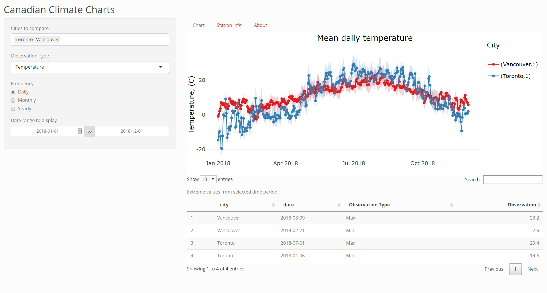
App Landing Page